The kinematics and dynamics of non-Cartesian actuators and robotics
For years, most motion system designers wanting to create motion in a 2D plane or in 3D space would use a Cartesian mechanism. The perpendicular action of Cartesian actuators makes several things easy for the system designer.
• First, Cartesian coordinates are commonly used and familiar.
• Second, having Cartesian actuators provides for a direct mapping of tool coordinates to actuator positions.
• Third, the same direct mapping applies to velocities and accelerations, making these easily calculable (and limitable) for each actuator. In addition, perpendicular Cartesian actuators create no significant dynamic interaction between the axes, so simple single-feedback control loops can be used on each axis.
• Finally, there is virtually no change in system dynamics over the travel of the actuators because the moment of inertia experienced by each actuator essentially stays constant.
However, modern computing power and controller technology are making it so non-Cartesian actuators can be used where they weren’t feasible or cost-effective before.
This in turn permits a great deal more choice in the physical configuration of mechanisms, often yielding startling increases in performance. How are all these benefits of Cartesian systems outweighed by alternative configurations?
Well, Cartesian systems do have their limitations. In almost all Cartesian mechanisms one axis carries another perpendicular axis; this requires much greater power and can yield lower performance for the carrying axis than other methods. Too, Cartesian mechanisms don’t produce the extended working area that serial-link mechanisms can provide (the area possible with a standard robot arm, for example.) Nor can Cartesian systems increase mechanical stiffness and reduce measurement errors as hexapods and other parallel-link mechanisms do.
Kinematics of the application we're considering
To maximize non-Cartesian system performance, full exploration and definition of the kinematic situation is required.
The subject of applied kinematics deals with the geometric relationship between a mechanism’s tool tip (or end effector) and the underlying linear and rotary joints that cause its movement. A forward-kinematic transformation computes the tool-tip coordinates from the joint positions. Conversely, the inversekinematic transformation computes the joint position from the tool-tip coordinates. Both of these transformations are needed if the end-user wants to program motion in tool-tip coordinates.
The forward-kinematic calculations must be done at the outset when starting from an arbitrary configuration to establish the starting tool-tip coordinates for the initial move. The inverse-kinematic calculations must be done at least for the end point of every move.
If a controlled path is also desired, these calculations must also be done at closely spaced intervals along that path.
Kinematic mechanism analysis
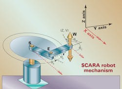
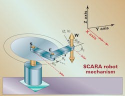
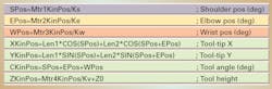
As an example, let’s consider the common SCARA robot. This mechanism has three parallel rotary joints turning about vertical axes — shoulder S, elbow E, and wrist W — and a single linear joint V in the vertical direction. The tool tip therefore has four degrees of freedom: three translational (X, Y, Z) and one rotational (C rotating about Z).
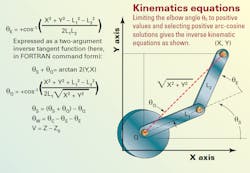
Limiting ourselves to positive values of the elbow angle θE that produce the right-armed case (done by selecting the positive arc-cosine solutions) we can write the inverse-kinematic equations as shown in the figure here.
Even this simple mechanism brings to light a couple of tricky issues commonly encountered with non-Cartesian mechanisms. The first problem is that there can be multiple solutions to the inverse-kinematic transformation: in this case, the right-armed and left-armed configurations. (Here, “right-armed” refers to the counterclockwise bend of the elbow joint, which looks like a human’s right arm from the top view.) Some method must be used to select which is used.
Also, there are some cases for which there are no possible solutions, no matter how far the joints can move. These must be handled — in this particular case, by recognizing that the argument for the arc-cosine function is out of the valid range of 1.0, as would happen at a physically unreachable tool-tip position. When the arc-cosine result for a certain input is invalid, it implies that the arms can’t move to that point.
Kinematic algorithm implementation
The inverse-kinematic algorithms should be embedded in the controller as subroutines, so they’re automatically called at the proper times to execute the transformation. This program can then work in the background to make it easier for end-users to use the final system, by allowing instructional input in tool-tip coordinates as if it were a Cartesian system.
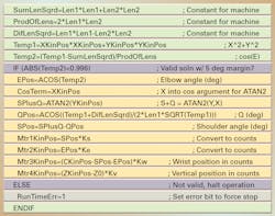
Let’s say you wanted to program your controller to first recognize the tool-tip position you’re starting with. The forward-kinematic subroutine for computing this would calculate that start point using the four motor (joint) positions, as shown below.
The inverse-kinematic subroutine computing the four motor (joint) positions could be programmed with the code shown above. The selection of the right-armed configuration is implicit by use of the positive arc-cosine solution; the checking for out-of-range solutions is explicit. The first three quantities computed are constant for the mechanism, and so do not have to be computed each time the subroutine is run.
Kinematic algorithm execution
What if the tool-tip path is also important? The amount of path accuracy required determines the frequency at which the inverse kinematics must be calculated. In our example, a coarse interpolation is first made in the tool-tip coordinates from the tip’s move specification (for example, a lin
ear or circular move) that yields intermediate tip coordinates along the programmed path. Next, these intermediate tip coordinates are passed through the inverse- kinematic algorithm to derive corresponding joint positions. Finally, a simple fine-motion interpolation algorithm computes intermediate points between these joint positions at the servo update rate, creating an approximation of the truly desired path.
The closer together the coarsely interpolated points are, the more accurate the resulting path will be. Almost never is it worthwhile to compute the kinematics every servo update, because separate fine-motion interpolation algorithms is so effective at smoothing motion into desired paths. However, it must be kept in mind that with more coarse interpolation points also comes a heavier load on the processor, because the inverse kinematics are a dominant computational issue. The typical period between kinematic updates is 5 to 10 msec.
In a mechanism such as this, the relationship between the tip velocities (and accelerations) and the underlying joint velocities (and accelerations) is strongly nonlinear, and varies over the course of a move. It is therefore very difficult for a user to predict with common methods when a desired motion would cause a violation of joint capabilities, leading to violent motion and possibly an error shutdown. This hinders full optimization of mechanism productivity.
On the other hand, sophisticated controllers can now monitor the resulting joint trajectories continually for potential violations of joint capabilities anywhere along the trajectories, slowing the trajectories of all joints together in a coordinated fashion (when needed) so that the limits of each are always observed. Because these very same limits also prevent instantaneous deceleration to required lower speeds, these algorithms scan ahead in the trajectory to detect violations, then work backwards from those points to calculate a feasible deceleration to the lower speeds. For this reason, these routines are commonly called look ahead algorithms.
Mapping the SCARA robot's dynamics
Besides full definition of the kinematic situation, the dynamic situation must be fully outlined to maximize non-Cartesian system performance.
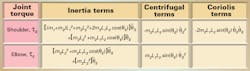
The SCARA robot we’ve explored here can also be used to illustrate special dynamic issues found in non-Cartesian mechanisms. The main dynamics challenge is that the dynamic equations can change significantly with the position of joints — particularly the elbow joint in this case — and the velocity and acceleration of one joint can affect the torque required for another.
The basic terms that contribute to the required torque for the joints are charted in the table at left; it shows the basic terms that contribute to the required torque for the shoulder and elbow joints. The upper and lower arms have masses m1 and m2, respectively, and lengths L1 and L2. The terms are broken into three categories: inertia terms, centrifugal-force terms, and Coriolis-force terms.
In reality, the moment of inertia is mL2/3 if the mass were assumed evenly distributed along the length. For simplicity however, the mass of each link is assumed to be concentrated at the far end of the link, giving an mL2 term for the moment of inertia.
Some of the inertia terms would be present in a Cartesian system as well.
However, other terms are unique to non-Cartesian systems. In the inertia terms, we see the torque at one joint dependent on the acceleration of the other joint. This is due to classic Newtonian third law of action and reaction. Also, the moment-of-inertia values are at least partially dependent on the angle of the elbow joint. The more the lower arm is extended at the elbow, the larger the moment of inertia becomes about the shoulder.
In addition to these forces are the effects due to centrifugal and Coriolis forces. The centrifugal terms on one joint are proportional to the square of the velocity of the other joint, and are at a maximum when the two links are perpendicular. The Coriolis term is proportional to the product of the two joint velocities, and is also at a maximum when the two links are perpendicular.
In most controllers, the servo loop for each axis (really, each joint) is closed independently, without regard to the action of other axes. Effects caused by other axes are just treated by the servo loop as disturbances to be rejected. But of course, before they can be rejected, they must create real errors in the axis — which can compromise the quality of motion.
In more sophisticated controllers these predictable interaxis effects can be used as cross-coupled feedforward terms. The purpose of feedforward is to anticipate the required torque for a given trajectory, leaving the feedback loop to handle only unanticipated disturbances and errors in the prediction. Most widely used are single-axis feedforward terms based on one axis’ own trajectory — particularly its velocity and acceleration feedforward components. The same principle can be extended to the dynamic effects on cross-coupled axes.
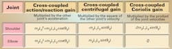
Employing cross-coupled feedforward terms using the instantaneous commanded velocity and acceleration of the other axis in addition to the standard feedforward terms dramatically reduces the disturbances induced by these effects. This can lead to more accurate actual trajectories or even increased dynamic capabilities while maintaining a given level of accuracy. Tables above show the cross-coupled gain terms required for this mechanism.
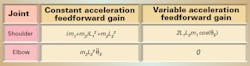
In addition to the standard, constant moment-of-inertia terms that can be multiplied by the commanded acceleration to produce an acceleration-feedforward term (as in a Cartesian system), our example SCARA robot also has a variable component in its moment of inertia about the shoulder joint. As already mentioned, it changes with the angle of the elbow joint. This means that every elbow movement changes the optimal acceleration feed-forward gain. The table below shows the constant and variable components of the acceleration feed-forward gain for the shoulder and elbow joints.
A sidenote on adaptive control and gain scheduling — live and learn
In the academic world, much attention is focused on automatic adaptive control algorithms that attempt, at least, to continually identify changing system characteristics from servo performance, and to adjust the gains accordingly. Most users in the industrial world don’t trust these types of algorithms, and for good reason; they often give unstable results by misidentifying the system parameters.
In industrial controls, a more popular method of adaptive control is the one we just explored — gain scheduling.
In this strategy, gain changes made are not based on closedloop performance, but rather in an open-loop fashion based on the system’s state. (In the case we just considered this is the elbow position and its resultant effect on the inertial moment about the shoulder.) While this might seem to be an inferior solution because there is no loop closed around the adaptation algorithm, it is more predictable because its possible range of actions can be precisely determined ahead of time.
Further, it cannot be fooled by unmodeled dynamics, as when friction is mistaken for higher inertia when movement is less than expected, for example. A controller that can directly compensate for these effects in non-Cartesian mechanisms can dramatically improve performance.
This capability is especially useful on wafer-handling robot arms. Due to the fragile nature of silicon wafers, end effectors cannot tightly grip them. To prevent dropping, smooth motion is critically important. The effects of the uncompensated dynamics have for a long time been a key limiting factor in the performance of these robots. Now however, implementation of the cross-coupled feedforward terms and scheduled gain terms yields dramatic improvements in performance of these systems.
For more information, visit deltatau.com.
About the Author
Curtis Wilson
V.P. of Engineering and Research
Delta Tau provided the first general-purpose motion controllers with on-board commutation for brushless motors, asynchronous PLC programs, DSP chips as the processor, digital current loops with direct PWM output, multi-move lookahead for robust acceleration control, and embedded kinematics algorithms for non-Cartesian mechanisms.
Elisabeth Eitel
Elisabeth Eitel was a Senior Editor at Machine Design magazine until 2014. She has a B.S. in Mechanical Engineering from Fenn College at Cleveland State University.
Voice Your Opinion!
To join the conversation, and become an exclusive member of Machine Design, create an account today!

Leaders relevant to this article: