Predicting downtime with intuitive software inspired by petrochemical process controls
Simple examples
To get a feel for the “values” produced by modern day MCM/PFA software, consider a few simple examples from the Tadpole system. The Tadpole algorithm is written in C. In these examples it ran on a National Instruments LabView software/cRIO hardware environment by virtue of a VI wrapper written around the Tadpole algorithm. The VI wrapper also simplified the Tadpole API to the two “values” of interest to MCM/PFA (Tadpole is designed with 25+ parameters for PID tuning and analysis). The VI runs in both the LabView Windows and LabView RealTime environments.
The first example is that of a single-frequency sine wave with slightly changing amplitude. It gives a high spectrum value because of the single dominant frequency and has a small error. Here the Spectrum value = 83.7 and the Error value = 2.86.
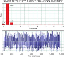
The second example is of a single-frequency sine wave with rapidly changing amplitude. It gives a high spectrum value because of the single dominant frequency with larger error value. The Spectrum value = 93.2 and Error value = 4.44.
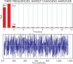
The final example is of three dominant frequencies with rapidly changing amplitudes. They give a low spectrum value of 13.7 with the same error value as above, 4.44.
Unfortunately, widely used machine condition monitoring/predictive failure analysis (MCM/PFA) software algorithms are complex. It takes highly trained individuals many hours to configure or analyze the results, while the software itself often gives marginal performance.
For example, one widely used MCM/PFA algorithm employs wavelet transforms. The problem is that wavelets require significantly high amounts of data and CPU horsepower to compute a solution, in many cases more than 10 megasamples and 20 to 30% of a quad-core CPU. Such horsepower is not economical when trying to use a programmable logic controller. Worse, wavelet transforms are sensitive to noise and other disturbances, and we all know noise-free data environments are virtually nonexistent in industrial settings.
Another problematic MCM/PFA technique employs neural networks that require training by historic or simulated data. This assumes that a model of the failure already exists. Unfortunately, there is no convenient library of failure models available for me, the “common man.” Neural networks also have the added expense of retraining each time a tuning parameter changes.
A third problematic MCM/PFA technique uses fuzzy logic. But fuzzy logic requires time-consuming custom coding/sequencing, usually by a subject matter expert whose time is expensive. And the predictions are only as viable as the fuzzy-logic rules. Worse, these algorithms become unpredictable or clamp when the data goes outside the range of the rules.
Likewise, Principal Component Analysis (PCA) and Singular Value Decomposition (SVD) are both linear MCM/PFA methods that don’t behave well in the complex nonlinear industrial world in which we work. Worse, their use demands that data of different scales must be normalized which generally trashes the minute details that help with the predictive analysis.
An “ideal” MCM/PFA technique would get around these problems and would require no coding, no extensive configuration, nor specialized training/education to operate. It would allow parameter configuration, by a junior engineer with no previous knowledge of the failure and detect trends,long before the high/low threshold alarms used on typical MCM/PFA data alerts. It would also provide a simple indication of a potential failure that could be evaluated by a junior engineer.
It turns out that the petrochemical process-control industry has evolved software along these lines. Pi Control Solutions LLC in Houston performs petrochemical control-system monitoring. It developed a proportional–integral–derivative (PID) tuning algorithm called True Amplitude Detection – Poles (Tadpole). Tadpole calculates about 25 “values” (simple integer numbers) representing the complex signals indicative of a PID used for closed-loop control of petrochemical processes. These values are generated by a detailed analysis of the complex data coming from the sensors. A change in one of these values indicates a change in the PID control quality.
We have found that two of the “values” produced by the Tadpole algorithm give an excellent representation of the complex signals indicative of a machine’s condition: The “Spectrum value” indicates the signal-frequency distribution. The “Error value” indicates signal amplitude.
A change in one of these two values indicates a change in the condition of the machine. These values stay in a fairly narrow range for a machine operating normally. This simplicity lets a junior engineer write simple code to look for a change in the “value.” Moreover, the junior engineer needs no prior knowledge of the data’s meaning, range, type, or proper value.
The Tadpole algorithm is particularly good at reliably detecting true oscillations on complex signals, handling real-time or logged data, and calculating the “value” with minimal data set. It works with any time period or data sample rate and can detect frozen signals (bad sensors), a rise in white noise (random noise) or jaggedness, and nonlinearities (the signal spending more time on one side of the mean).
The value of a Tadpole analysis becomes more clear by viewing a few examples of the “values” produced from simple signals. We set up various failure test cases using data logs from customer machine-monitoring systems. We recreated log data by running it through a National Instruments, Austin, analog output card. We then added various error signals to the logged data to create the controlled failure conditions needed for proper verification and validation.
Readers should note that we’ve exaggerated the inserted errors (oscillation, noise, modulation, etc.) in these test cases for clarity. We see more subtle errors in actual machine data.
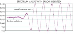
Predictive failure case 1 — Simple bearing oscillation detection: On the left side of the accompanying figure, the log data contains minor bearing noise (random oscillation), which provides a baseline spectrum “value” of 6.04. On the right side of the figure, a single-frequency sine-wave error is inserted, causing the spectrum “value” to rise to 32.13, which is easily detected as a bearing abnormality. This is significant because we did not need to configure the algorithm so it would look for specific spectral content or teach the algorithm to look for oscillation. We just fed data into the algorithm, and it identified a change in the bearing.
Predictive failure case 2 — Noise detection: The accompanying figure depicts our log data which contains minor compressor noise, giving a spectrum “value” of 12.67 and an error “value” of 0.27. The figure depicts the insertion of noise having essentially the same frequency as the data of interest. This causes the spectrum “value” to change slightly to 14.4, but the error “value” jumps significantly to 4.78, again easily detected as a compressor abnormality.
The error “value” changed significantly because of the change in amplitude, but there was a small change in spectrum “value” because the spectral content stayed close to the same. Had we simply added the baseline log data to itself, the spectral “value” would have remained the same.
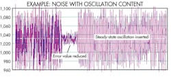
Predictive failure case 3 — Lack of Noise Detection: This test case demonstrates the crux of the errors most people encounter in cases where noise goes away (possible bad sensor) or when noise starts to show oscillatory content (possible machine failure). On the left side of the figure, the log data has typical noise (random oscillation), which provides a baseline spectrum “value” of 13.8 and an error “value” of 2.54. In the middle of the figure, we attenuated the noise which caused a significant drop in the error “value.” On the right side of the figure, the noise returns to the original level. But we inserted a steady-state oscillatory error, which caused the spectrum “value” to drop to 8.1 while the error “value” returned to its baseline state, easily detected as an abnormality. A smaller spectrum “value” means the signal is comprised of many different frequencies. In this case, a fast noise component was followed by a slower noise component which was followed by strong oscillatory component.
This response is significant because we did not have to configure the algorithm to look for oscillatory content within the noise or teach the algorithm to look for possible sensor errors. We just fed data into the algorithm, and it identified a change.
Predictive failure case 4 — Noise Detection on a Highly Oscillatory Signal: The first graph in the accompanying figure provides a data log with a blend of three high-frequency signals from a high-speed rotary-assembly machine, giving a spectrum “value” of 145.1. The second graph shows random noise introduced in the same frequency range and amplitude, giving a significant drop in the spectrum value to 9.59, again easily detected as abnormal. This result is significant because there was no need for a subject matter expert or spectral analysis to detect the problem. The tool itself identified the issue.
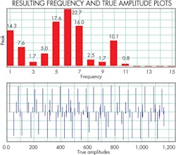
With the Chatter parameter set to its default, the value is 2.97 (relatively small, indicating the presence of several signal frequency components) as represented by several large and small blue bars in the accompanying figure.
To eliminate the high-frequency noise, the Chatter value is adjusted to 1.075 resulting in the blue bars showing just the low-frequency pure sine wave without the high-frequency noise (smaller blue bars are gone). The Spectrum value jumps from 2.97 to 18.3. This simple display lets even inexperienced personnel rapidly focus on data of interest.
With all these predictive failure cases the TadPole software is not a prognostics tool, it still takes a good engineer to design and recommend corrective actions. However, this is the best MCM/PFA tool we have found to analyze data quickly and economically.
This file type includes high resolution graphics and schematics when applicable.


