Analog lead-lag velocity control
This article concludes a two-part series on analog velocity loops. It addresses lead-lag velocity control, building on last month’s discussion on proportional-integral (PI) control loops.
By adding an RC circuit across the tachometer feedback resistor of a PI controller, it’s possible to improve system performance without a corresponding jump in cost. The parallel path produces a derivative term, which advances the phase of the loop. This advance or “lead” allows the proportional gain to be increased by about 40% and the integral gain can be strengthened even further. Higher gains naturally mean better command response and disturbance rejection. The drawback is that tuning is more complicated.
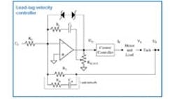
The control-loop diagram for a leadlag velocity controller is like that of an analog PI loop with the addition of a “filtered derivative” path representing RA and CA. The resistorRAprovides a low-pass filter through which the differentiated feedback signal from CA passes. Without RA, the derivative would be too noisy to be of any use in an industrial system. The presence of a derivative term explains why lead-lag is occasionally referred to as “PID” control.
Tuning a lead-lag controller is similar to tuning an analog PI controller. In both cases, you tune in zones (see Tune up, June 2000).
With lead-lag there are two zones – proportional and integral. As with a PI controller, apply a small-magnitude velocity step command to the drive, making the step as large as possible without calling for peak drive current. Next, adjust the zones one at a time. For Zone 1, zero the integral gain (short CL) and set RL as high as possible without generating overshoot. Next, increase RL by about 40%. This will generate overshoot that will be cured by the lead network.
The value of RA is a compromise between performance and noise. A smaller value means larger increases in RL, portional gain) but greater susceptibility to noise. A rule of thumb for servo systems is to set RA to about 1/3 the value of the tachometer scaling resistor RT.
To tune Zone 2, increase CL until the overshoot reaches 10 to 15%. Remember to set the RSCALE pot away from the ends of travel, so that if inertia varies in the future, you can use the full potentiometer range to maintain optimal tuning.
In addition to allowing about 40% higher proportional gain, lead-lag offers the opportunity for an even greater improvement in static stiffness.
Static stiffness is the resistance you feel from a servomotor trying to hold it’s position while you apply torque to the shaft by hand. It is the measure of the system’s ability to resist constant torque disturbances such as the effects of Coulomb (sliding) friction and gravity. With higher static stiffness, a machine is likely to be more accurate in the presence of constant disturbances.
The servo gain with greatest influence on static stiffness is the integral gain, set here by CL. Smaller values of CL produce higher static stiffness. In this lead-lag controller, for example, CL is adjusted to 0.004 μF; in the equivalent PI controller from last month, CL couldn’t go below 0.01 μF without generating excessive overshoot. So in this case, lead-lag helped reduce CL by 40%, producing about 2.5 times more static stiffness than PI control.
Tune time
Want to tune an analog lead-lag velocity controller yourself? Then log onto www.motionsystemdesign.com and download the most recent version of the ModelQ simulation program. Launch the program and select November’s model. Click “Run.”
This is the analog lead-lag controller discussed here. The command (blue) and response (black) are overlaid; current is shown below. During tuning, it’s always a good idea to monitor current to ensure the system stays out of saturation. As before, if you have questions about constants, click on the button “About this model....”
To tune the system, start in Zone 1. Set CL to 0 and adjust RL to where some overshoot starts to appear, then adjust it down. The highest value of RL where there’s no overshoot is about 500 kΩ. Next, raise RL by 40% to 700 kΩ in anticipation of the improvement that will be provided by the lead circuit. Set RA to 1/3 of RT or about 6.8 kΩ, and adjust CA to 0.005 μF to remove overshoot.
The final step is to add CL. Always start with a fairly large value, remembering that lower values of CL create larger servo gains. Here, a value of 0.005 μF gives a good step response — about 10% overshoot.
George Ellis is a senior scientist at Kollmorgen, Radford, Va. His latest book, “Control System Design Guide,” 2nd edition, was published in May, 2000 by Academic Press. He can be reached at [email protected].
About the Author
Voice Your Opinion!
To join the conversation, and become an exclusive member of Machine Design, create an account today!

Leaders relevant to this article: